Sample data, simple usage

Google Datalab and BigQuery are useful for image classification projects. We will start with a simple project here. First things first — Google Datalab is used to build Machine Learning (ML) models and runs on Google’s Cloud virtual machine. BigQuery is cloud-based big data analytics web service for processing very large read-only data sets, using SQL-like syntax. Basically, what previously might have been done on a pc or network computer using dedicated resources and an installed database, can now be accessed through a computer with an internet connection. All the heavy lifting and processing is done in the cloud to achieve the same result in a more efficient manner.
Before you begin, ensure that:
- You signed on to a Google Cloud account.
- Google Compute Engine VM is created and active.
- Machine Learning and Dataflow APIs are enabled.
- You have an active project, Datalab and an active notebook.
If you are not sure how to do any of the above, there are several good articles that show you how — here’s one: https://towardsdatascience.com/running-jupyter-notebook-in-google-cloud-platform-in-15-min-61e16da34d52.
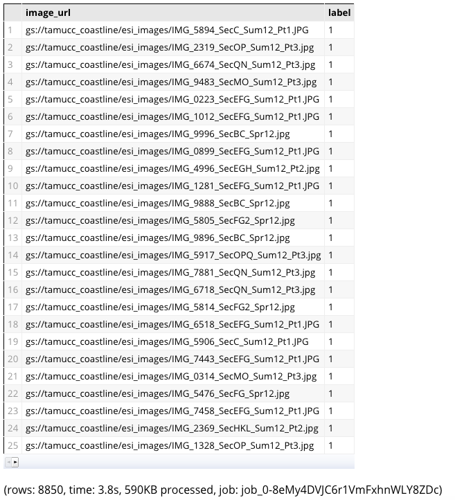
Acknowledgement: The images and the code example are from Google Datalab samples, with my explanations added. The images are from low-altitude aerial photography of Texas shorelines, and the purpose of the program is to predict the type of images of the coast (tidal flats, man-made structures etc.) that are the main composition of this library. Link: gs://cloud-datalab/sampledata/coast. https://storage.googleapis.com/tamucc_coastline/GooglePermissionForImages_20170119.pdf for details.
These are the steps we will take:
- Define a BigQuery dataset — define a name, and create a schema (structure definition with field names and types)
- Create tables for training and testing / evaluation
- Import data from existing BigQuery tables (training, evaluation) that contain image files, to the dataset’s tables
- Run the job to create the BigQuery dataset
- Execute the dataset to populate tables with existing Google data
- Review the data by creating histogram plots for training and testing (evaluation) data
Start a new notebook file and input:
#point to a Google storage project bucket, will use your project id
bucket = 'gs://' + datalab_project_id() + '-coast'
#make bucket if it doesn't already exist
!gsutil mb $bucket
Load the data from CSV files to Bigquery table.
import google.datalab.bigquery as bq
# Create the dataset
bq.Dataset('coast').create()
#create the schema (map) for the dataset
schema = [
  {'name':'image_url', 'type': 'STRING'},
  {'name':'label', 'type': 'STRING'},
]
# Create the table
train_table = bq.Table('coast.train').create(schema=schema, overwrite=True)
#load the training table
train_table.load('gs://cloud-datalab/sampledata/coast/train.csv', mode='overwrite', source_format='csv')
#create the eval table
eval_table = bq.Table('coast.eval').create(schema=schema, overwrite=True)
#load the testing (evaluation) table
eval_table.load('gs://cloud-datalab/sampledata/coast/eval.csv', mode='overwrite', source_format='csv')
Type the following for the label description:
!gsutil cat gs://cloud-datalab/sampledata/coast/dict_explanation.csv
output:  (label code and description)
class,name
1,"Exposed walls and other structures made of concrete, wood, or metal"
2A ,Scarps and steep slopes in clay
2B ,Wave-cut clay platforms
3A ,Fine-grained sand beaches
3B ,Scarps and steep slopes in sand
4,Coarse-grained sand beaches
5,Mixed sand and gravel (shell) beaches
6A ,Gravel (shell) beaches
6B ,Exposed riprap structures
7,Exposed tidal flats
8A ,"Sheltered solid man-made structures, such as bulkheads and docks"
8B ,Sheltered riprap structures
8C ,Sheltered scarps
9,Sheltered tidal flats
10A ,Salt- and brackish-water marshes
10B ,Fresh-water marshes (herbaceous vegetation)
10C ,Fresh-water swamps (woody vegetation)
1OD,Mangroves
BigQuery — create the query; notice it is similar to SQL
#create the query - --name, then the actual name, then SQL like statement %%bq query --name coast_train SELECT image_url, label FROM coast.train
#execute the query
coast_train.execute().result()
Sample the data to around 1000 instances for visualization. Our data is very simple, so we simply draw histogram on the labels and compare training and evaluation data.
#import ml libraries and functions
from google.datalab.ml import *
#set labels (names) for the datasets with the tables for training, eval
ds_train = BigQueryDataSet(table='coast.train')
ds_eval = BigQueryDataSet(table='coast.eval')
#sample of training and eval data, for simple example - 1000
df_train = ds_train.sample(1000)
df_eval = ds_eval.sample(1000)
#plot a bar chart for the training values
df_train.label.value_counts().plot(kind='bar');
#plot a bar chart for the eval (test) values
df_eval.label.value_counts().plot(kind='bar');
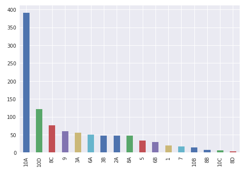
Bar chart showing type of image at bottom (x-axis) and # of image files on left (y-axis) for TRAINING
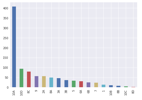
Bar chart showing type of image at bottom (x-axis) and # of image files on left (y-axis) for TESTING / EVAL DATA
Notice that the data is similar for both, as this is a small sample and a simple evaluation case. Most of the image files are of type ‘10A’ — Salt- and brackish-water marshes. This can be expanded to create a model and do more intensive classification for better predictions.
This article is also published on Medium.com here:https://medium.com/@hari.santanam/using-google-datalab-and-bigquery-for-image-classification-comparison-13b2ffb26e67