Using Keras to predict fashion dataset and see images used by machine learning
AI uses Image recognition learning processes to go through thousands of images and “learn” which images belong to which category. My example program uses the MNIST fashion dataset to sort through thousands of images of clothing types (jackets, shirts, pants, dresses etc.) and accessories (handbags, shoes etc.) to classify the images into their proper categories; the program also saves the model and then re-uses it. I also use a key-value pair process to map the clothing code to the description and loop through samples of the testing data to pull and view some of the images and the predictions for those images. Here is a summary, which most are already familiar with:
1. import the libraries and modules - tools required to run the program.
2. load the mnist fashion dataset into x_train, y_train, x_test and y_test sets - divides the data into training (used by program to learn) and test (program tests its predictions against test data and gets better at learning for optimal results based on defined parameters).
3. preprocess the data and class tables - turns the datasets into more standardized, program readable sets.
4. Define the model architecture - tell the program which parameters to use and methods to use for learning; define the input shape.
5. Compile the model - configure the learning process for the program.
6. Fit the model to data - run the model on the data.
7. Save the model for future use - (I saved the model on first run and re-used it on subsequent runs, commenting out the save step).
8. key-value pair - map the label code to a description that people can make sense of (e.g., 4 = Coat, 8 = Bag).
9. added a range - pulled out sample images from the test data to view the image and the program's prediction of what the image is.
The code is listed below; if you are more interested in parts 8 and 9 (key-value pair and view sample of test image files and predictions), scroll down.
(1) Load and import functions
from keras.models import Sequential
from keras.layers import Dense
from keras.utils import np_utils
from keras.optimizers import SGD
from keras.datasets import fashion_mnist
import matplotlib.pyplot as plt
(2) Load fashion dataset into training, testing sets and print their dimensions
(x_train, y_train), (x_test, y_test) = fashion_mnist.load_data()
print(x_train.shape)
print(y_train.shape)
print(x_test.shape)
print(y_test.shape)
(3) Preprocess data and class labels
x_train = x_train.reshape(60000, 784)
x_test = x_test.reshape(10000, 784)
y_train = np_utils.to_categorical(y_train, 10)
y_test = np_utils.to_categorical(y_test, 10)
(4) Define the model architecture
model = Sequential()
model.add(Dense(units=128, activation="relu", input_shape=(784,)))
model.add(Dense(units=128, activation="relu"))
model.add(Dense(units=128, activation="relu"))
model.add(Dense(units=10, activation="softmax"))
(5) Compile the model
model.compile(loss="categorical_crossentropy", optimizer=SGD(0.001), metrics=["accuracy"])
(6) Fit the model
model.fit(x_train, y_train, batch_size=32, epochs=10, verbose=1)
(7) Run the model (note: save it the 1st time, like below)
model.save("mnist_fashion_ds-1.h5")
(7a) Run the model (from 2nd time onwards — ensure that the path is correct!)
model.load_weights("mnist_fashion_ds-1.h5")
(8) Key-value pair: A map for easy readability: Descriptions are easier for humans :).
d = {0:'T-shirt/top',
1: 'Trouser',
2: 'Pullover',
3: 'Dress',
4: 'Coat',
5: 'Sandal',
6: 'Shirt',
7: 'Sneaker',
8: 'Bag',
9: 'Ankle boot'}
(9) range (for loop) to select several image sample files from the test dataset, and have the program predict what image it is, and print the image as well to see for ourselves.
for x in range(100,4000,200):
  img = x_test[x]
  test_img = img.reshape((1,784))
  img_class = model.predict_classes(test_img)
  classname = img_class[0]
  print("Class: ", classname, d[classname])
  img = img.reshape((28, 28))
  plt.imshow(img)
  plt.title(classname)
  plt.show()
Once this is created, compiled and run, you should hopefully have output like this — (1) watch the epochs run and get some accuracy and loss figures, and (2) see some sample images and predictions like this:
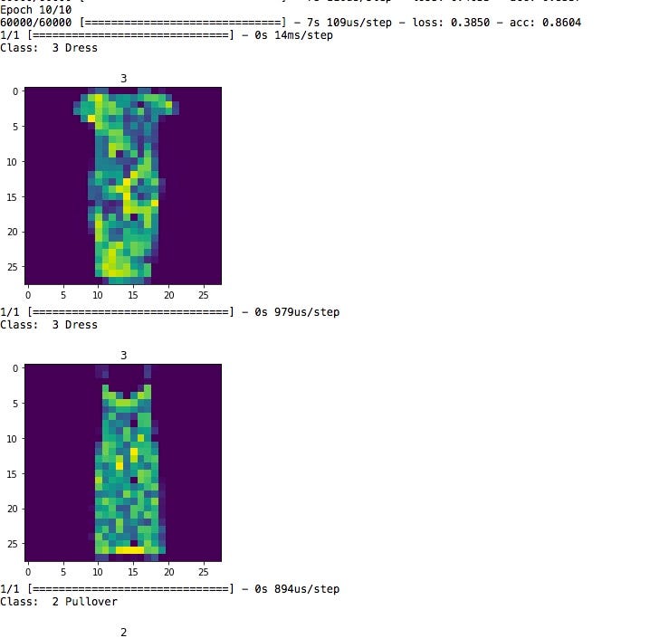
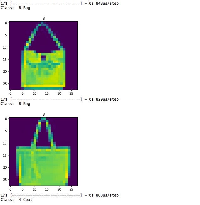
It is good to see some samples and predictions paired with the images, as these programs can get complicated as they scale up. Visualizing makes it easier to understand, I think. I broke the code into snippets for better explanations.
This article is posted on here on Medium as well
This article is posted on here on Medium as well